Last month, climate scientist Kate Marvel, of NASA, shared “something I have really struggled with” about extreme event attribution. She was speaking as an invited expert in a public information-gathering session of the U.S. National Academy committee1 on extreme event attribution.
Marvel, who also served at the lead author on the chapter on “Climate Trends” in the 2023 U.S. National Climate Assessment,2 explained to the committee that her struggle resulted from the seemingly contradictory findings of (a) the IPCC — which does not detect long-term trends in most metrics of extreme weather, and (b) claims made of extreme event attribution — which seem to find large changes in just about every type of extreme weather:
There’s not [in the IPCC] a lot of “we have a really robust attribution of these long-term trends to human activities,” and that might seem to fly in the face of, “OK well this heat wave is X% more likely or severe or whatever due to human activities.” That’s something I have really struggled to bridge when I’m talking to the public.3
Marvel’s struggle is real.
As I have documented extensively here at THB, the findings of the IPCC on detection and attribution are indeed at odds with the headline-generating pronouncements of the extreme event attribution community. Reconciling the differences between the two does not however require a struggle.
The IPCC has for decades played things (mostly) straight in assessing the peer-reviewed literature on detection and attribution associated with extreme weather events. In contrast, extreme event attribution is alchemy conjured up largely outside the peer-reviewed literature and promoted via press releases.
Today’s post pulls back the curtain on World Weather Attribution (WWA), which is surely one one of the most successful marketing campaigns in the history of climate advocacy. I call it a marketing campaign based on how they describe their goals:
- “[I]ncreasing the ‘immediacy’ of climate change, thereby increasing support for mitigation”
- “Unlike every other branch of climate science or science in general, event attribution was actually originally suggested with the courts in mind”
WWA has found considerable traction despite its disdain for peer-review — its press releases generate headlines around the world, show up in legal filings, and are even widely cited in the peer-reviewed literature. WWA is also central to the current National Academy of Sciences/Bezos Earth Fund extreme event attribution study — which has the same funder as WWA and membership on the committee itself.
If you read the first five parts of this THB series on Weather Attribution Alchemy, you’ll quickly learn that my concern is not to quibble about the small methodological details of extreme event attribution. Rather, my critique is that extreme event attribution is pseudoscience, seemingly created to undermine the scientifically robust detection and attribution framework of the IPCC.
Despite its public relations successes, few know what WWA actually does and how it does it in linking seemingly every notable weather event to climate change (and as THB readers know, climate change is not a cause). This is the first of two posts describing the methods of WWA and how those methods are used to generate eye-popping results that make headlines around the world.
The approach used by World Weather Attribution to identify the “effect of global warming on recent extreme events” has, by their accounting, eight steps.
The first is to identify an event that has just happened with some sort of notable impact. The second step involves identifying a specific variable to characterize the event and on which to center the analysis — such as daily high temperatures over 40C or maximum five-day rainfall each year.
The third step is crucial, and the focus of this post:
The next step is to analyse the observations to establish the return time of the event and how this has changed. This information is also needed to evaluate and bias-correct the climate models later on, so in our methodology the availability of sufficient observations is a requirement to be able to do an attribution study.
Both sentences here are important, the observational time series serves two purposes — (1) establishing how the extreme event has changed (i.e., establishing a trend), and (2) serving as a filter to select which model runs are deemed relevant to making attribution claims.4
How long a time series is required to adequately determine the return time of the event? WWA explains that,
A long time series is needed that includes the event but goes back at least 50 years and preferably more than 100 years.
The statistics of the observational time series are assumed to be characterized by an extreme value distribution (and it appears that the generalised extreme value (GEV) function is typically preferred in WWA studies). If you are interested in a fantatsic short (~7 minute) tutorial on GEV, click on the video below.
WWA makes two further assumptions that are fundamental to their methodology and their results, first:
- “[T]he distribution [of historical observations] only shifts or scales with changes in smoothed global mean surface temperature (GMST) and does not change shape”
This means that the distribution of the relevant variable is assumed to be stationary (unchanging) except for the influence of changes in global mean surface temperature. There are three huge problems with this assumption.
First, smoothed (i.e., multi-year averaged) changes in GMST do not “influence” weather — GMST is a metric that integrates temperatures in locations around the world, and a multi-year average integrates the metric over time as well as space.
Second, an assumption of stationarity necessarily implies that the distribution fitted to an observational record accurately reflects the entire scope of natural variability — if it did not, then any trends in an observational time series could be the result of variability on longer time scales than that of the observational dataset. The WWA methodology assumes that 50 to 100 years is sufficient for encompassing natural variability. This assumption is incorrect, according to the IPCC.
Third, restricting a shift or scaling change in GEV only to GSMT means that any such change in a distribution is necessarily due to GMST — Attribution achieved! That which was to be proven is simply assumed.
This problem has been recognized in a more technical description of the WWA methodology:
Note that while using smoothed global mean temperature we cannot attribute changes to local forcings, such as aerosols, irrigation, and roughness changes, which can also have large influences on extremes (Wild, 2009; Puma and Cook, 2010; Vautard et al., 2010). This should always be kept in mind and checked when possible. If factors other than global warming are important for changes in the distribution, attribution to global warming alone is not appropriate and additional investigation should be conducted. See for instance the analyses of heat in India, in which air pollution and irrigation are as important (van Oldenborgh et al., 2018), and of winter storms in Europe, where roughness appears to be much more important than climate change (Vautard et al., 2019), but also land surface changes in heat extremes in the central US (Cowan et al., 2020).
In practice, such considerations fail to receive much if any attention in the WWA press releases and headlines.
The second WWA assumption reinforces assumed attribution:
- “[G]lobal warming is the main factor affecting the extremes beyond year-to-year natural variability . . . For many extremes, global warming is the main low-frequency cause of changes, but decadal variability, local aerosol forcing, irrigation and land surface changes may also be important factors.”
In looking at a time series of a relevant variable, WWA asserts that they must determine “whether there is a trend outside the range of deviations expected by natural variability.” I have read dozens of WWA studies for this post and I have not seen one that evaluates whether an asserted trend lies outside the range of expected natural variability.5
Consider the example below from a WWA attribution analysis of extreme rainfall in Botswana and South Africa.
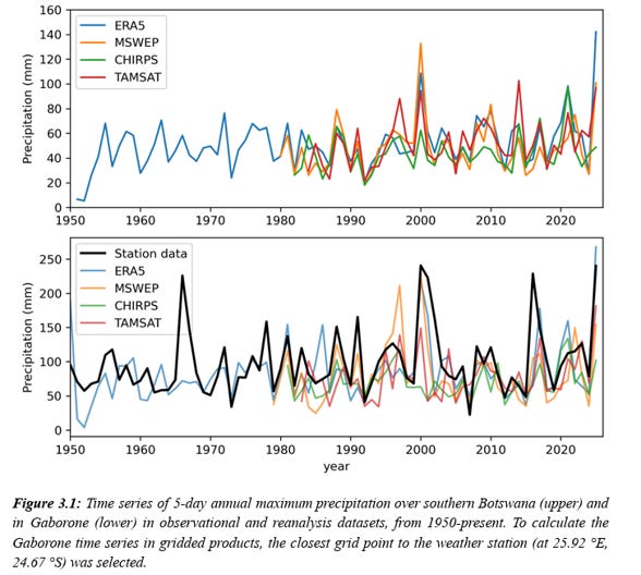
WWA asserts of the time series shown above:
“All observational datasets used in this study give strongly increasing trends in the rx5day index due to current warming of 1.3 °C, both at the region scale and at the scale of a single grid point or weather station.”
Really? Not only does this claim fail a natural variability eyeball test of the time series in the figure above, it presumes to conclude the point of the analysis, which is attribution. In this study, WWA does not assess whether the purported trends in the time series above lie outside natural variability.
Across WWA studies, observational data is treated in a seemingly arbitrary manner. Below are just a few examples from recent studies.6
Mediterranean 2023: The WWA acknowledges that “no discernible signals in heavy precipitation for the region overall.” However, in its analysis WWA generated a trend by eliminating use of one dataset based on a claim that the record was too short (1979), leaving only a dataset with a trend, contrary to the broader published literature and data.
“due to the short length of MSWEP [44 years, from 1979] we use the longer ERA5 dataset [73 years] as our primary source for the observational analysis of Rx4day over the GBT region”
Consider also that four other WWA studies — Argentina, Botswana, Sudan, and Nepal — used 16 datasets (some are used in multiple studies) and 11 of these dated from 1979 or more recently, with shorter time series often preferred over longer ones.
Argentina 2024: Four of the datasets used in this study showed a decreasing likelihood of extreme rainfall in the relevant region. No matter! An attribution claim was made instead based on a bespoke collection of five individual weather stations, only one of which WWA reported having a statistically significant trend.
“Compared to the preindustrial climate, the current warming level has resulted in a decrease in the likelihood of extreme rainfall events such as the one under study . . . based on the ERA5, MSWEP, CPC and CHIRPS datasets . . . On the other hand . . . results from analysing the trends at stations in five locations in the study region- namely, Bahía Blanca, Dolores, Santa Rosa, Bolívar and Córdoba . . . suggest that extreme rainfall in the region is increasing in response to global warming.”
Central Europe 2024: After publication, WWA acknowledged that it had made a significant error in how it characterized a trend in one of the datasets that it used — It was in fact a huge error, an order of magnitude.
“The change in intensity in the E-OBS dataset was erroneously reported as an increase of 50%, when it should have been an increase of 5% . . . and do not affect the . . . the overall conclusions of the study.”
In its correction, WWA dropped another dataset with no trend and also claimed that the large error was irrelevant to the study’s conclusions. That says something about the sensitivity of WWA conclusions to observational inputs.
What an early peer reviewer of WWA research said of its approach: “Frankly speaking, I do not see much robust added value beyond a simple generic Clausius-Clapeyron argument that any climate scientist could have given to the media while the event was unfolding. The whole method intercomparison framework seems to imply a rigorous scientific assessment of an accuracy that goes far beyond such a general thermodynamic argument. But does it really do so? I am not convinced, maybe because, at most, the manuscript meets the standards of a blog article rather than the ones of a scientific paper.”
Reviewer #7 on an early (2016) WWA paper submitted to a peer-reviewed publication. The paper was rejected. Not long after, WWA announced that it would not seek to publish in the peer-reviewed literature and instead would focus on getting into the media. It worked!
A remarkable example of arbitrariness in trend identification is Nepal 2024, which is worth explaining in some detail. In this study, WWA included two time series of the ERA5 dataset, one dating to 1950 — and showing no trend — and one from 1979 showing a significant trend.
WWA explains:
“[O]ne data set, ERA5, is included twice, from 1950, the start of the available time series, and from 1979, the beginning of the satellite era. This is to highlight that the trends change in sign, depending on the length of the timeseries but also distorts the relative weighting of the available data.”
Unlike the Mediterranean example above, in which a dataset from 1979 (too short!) was discarded in favor of one from 1950, in the Nepal study time series from both 1979 and 1950 are included and weighted the same — and even worse, they are the same data!
Of the other two datasets beyond ERA5 considered in the Nepal analysis, one showed a trend of increasing extreme rainfall and the other decreasing, so they cancel each other out. With the ERA5 from 1950 showing no trend, that means the use of the truncated series from 1979 was the deciding factor for the results. Clever!
Further — because the truncated ERA5 dataset was a subset of a the time series showing no trend, that means that the trend of truncated ERA5 time series was — by definition — not outside the range of natural variability, contrary to how WWA describes its approach, and should not have been used.
With a trend in hand, WWA’s next step is to regress the variable of interest (or an index thereof) on global mean surface temperature. You can see that below from the Nepal study, showing an index of 3-day accumulated precipitation (Y-axis) against a four-year average of global mean surface temperature.7
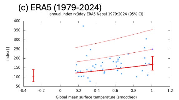
Since global temperatures have increased since 1979, any trend in the observational dataset will result in a linearly increasing regression, purportedly indicating the degree to which increasing smoothed global temperatures are associated with an increase in extreme values in the observations. Establishing that relationship is why trend identification is so important to the WWA methodology.
The figure above shows, with the vertical red lines, that extreme rainfall in today’s climate (at about 1.0 on the X-axis) is much higher than in a pre-industrial climate (at about -0.3 on the X-axis), established by simply extending the linear relationship from the short time series backwards to the pre-industrial era.8
The difference between today and pre-industrial is then used to create two different estimates of return periods for different levels of 3-day extreme rainfall in Nepal — simply by shifting the distribution of observed events by the difference between the two vertical red lines in the graph above. The result is shown below.
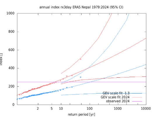
The figure above shows — with the purple horizontal line — that a 100-year flood in the pre-industrial climate would be about a ~5-year flood in 2024, or 20 times more likely. There’s the headline!
This result then drives the selection of which climate models are appropriate to use in the analysis — model runs that support this result are selected and those that do not are tossed (more on that in a follow up post). Clever, no?
WWA explains their approach in the one-minute (and silent) video below, prepared associated with their analysis of a Mediterranean heat wave.
Back to the Nepal example — What do the two graphs above look like if instead of the truncated ERA5 dataset from 1979, WWA instead uses the full ERA5 time series from 1950?
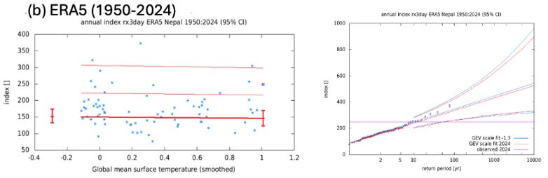
No attribution, and a completely different basis for selecting model runs that support this conclusion.
WWA researchers select the event, the variable used to represent the event, the spatial scale over which the variable is measured, the dataset(s) used to measure the variable, the length of time series, and which time series are included or discarded.9 Of course trends can be readily identified related to specific extreme weather phenomena and for which the IPCC has not achieved detection or attribution.
No struggle needed — weather attribution alchemy!
What about those rare cases where WWA simply cannot identify trends in extreme weather related to the event? No worries, models to the rescue. Next time . . . we will look at how WWA uses climate models to reinforce or repair conclusions derived from observational data.
This post originally appeared on The Honest Broker. If you liked this post, please consider subscribing here.
1 This is the same committee compromised by incredible conflicts of interest that I discussed in an earlier post in this series.
2 Marvel’s chapter in the NCA led with NOAA’s “Billion Dollar Disasters” as primary evidence of trends in extreme weather events, but I digress.
3 Marvel’s comments come after ~2:44 in the video of the event.
4 I’ll discuss the use of models in the follow-up to this post, but careful readers can anticipate the methodological issues that result from cherrypicking a subset of model runs based on expecting them to support a predetermined conclusion.
5 The IPCC faces challenges achieving detection of change at the global scale for most types of extreme weather, at local scales it is much more difficult.
6 The list of examples could be much longer, these are simply from the first studies I looked at.
7 Correlations using smoothed data are, ahem, problematic. For another day.
8 The lowest line is used here by WWA because it lies at the 95% confidence interval.
9 I assume here that all WWA researchers are working in good faith. One can make their way through a garden of forking paths in many ways.